In this post, I use some lecture notes from an online course/talk about “Modern Time Series Analysis” presented by Aileen Nielsen in Scipy2019 and format them to produce a written tutorial for people interested in this topic.
Introduction
Main steps in time series an:
- Visualization (seasonality, stationarity)
- Indentifying/modelling undernying distributions of data and stochastic process generating the data.
- Smoothing (past), Filtering (present), Forecasting (future)
- Classification
- Anomaly detection, outlier points within time series
Some examples of time series analysis systems:
- Let’s suppose we perform a noisy measures, time series analysis can allow to estimate what was the true value given these noisy values.
- Classification of healthy and unhealthy EKG signals.
- Anomaly detection of bank card fraud or dysfunctionning of some industrial facility
A note on Cross-sectional vs Time series:
- More missing data in time series;
- High correlation between timesteps;
- Timestamps can be used as a measure of distance.
One axis is monotonically increasing (time axis) The signal can show some charesteristic such as seasonality, cycles, autocorrelation & trends. It is also possible to spot some stochastic shift to some specific stochastic regime.
Frequent problems with time series:
- Residuals of time series models significance (special time-aware diagnostics/evaluation, autocorrelation plot of the residuals)
- Cross-validation depends on the data and on the future does not leak backwards in time and overestimate your model performance. CV should roll test and train forward in time. In other words, we avoid to test on data that is older (in time) than train data.
- Lookahead is another issue, timestamping does not mean when you would actually have that data points. Sometimes, this is not an issue.
State Space Models: Box-Jenkins ARIMA as an example
BJ-ARIMA (autoregressive integrative moving average,same classe of AM, ARMA for AutoRegressive-Moving Average):
- Remarkably successful to model basic timeseries a yields cutting edge performance
- Particularly effuicient on small datasets with no too much noise and some seasonalit
We choose this model because it is quite performant for a bunch of problems. It is also not the most simple one but it made of simpler components that we will describe as we go along.
ARMA Model
Here is the mathematical formulation of the ARMA model:
where $\alpha_{1:p}$ are called autoregressive components, $\theta_{1:q}$ are the moving average components and $L$ is called a lag operator that moves a variable back (or forth) in time. The lag operator of power $2$ transforms $X_t$ to $X_{t-2}$. In this type of models, future values depends past values and past errors. $p$ and $q$ are the main parameter to fiddle with to tune the model.
ARIMA Model
Now, let’s look at the mathematical formulation of the ARIMA model:
The difference with ARMA is the term $(1-L)^d$. Mathematically, this makes the future values depend on $\Delta X$ instead of $X$ values. The only lost information is the offset, but makes the model more tractable.
Fitting these models is not a trivial task (is more like an art).
Limits of ARMA/ARIMA
- These model are not especially intuitive
- No way to build an understanding about how it works (Random walk, cyclical elements, external regressors)
- Some systems we try to model present slow or stochastic cycle that cannot be taken into account with ARIMA models (e.g. a cycle of 24 hours in hourly data can be hard to spot and the model does not get better with more data).
Structural time series
let’s suppose a type of time series that can be split to multiple time components (a certain level/offset, seasonal/periodic, irregular/noise).
The structural time series can be expressed in ARIMA form, and can be fit via maximum likelihood estimator (see Kalman filter). The particular feature of there models is to offer insights into the underlying structure. (Also compatible with Bayesian analysis).
The 3 solutions offered by state space models
- Filtering: The distribution of the current state at time $t$ given all previous measurements up to and including $t$ (e.g. noise removal).
- Prediction: The distribution of the future states at time $t+k$ given all previous measurements up to and including $t$ (e.g., forecasting).
- Smoothing: The distribution of a given state at time $k$ given all previous and future measurements from $0$ to $T$ (e.g., correct past estimation given future values).
Kalman Filter
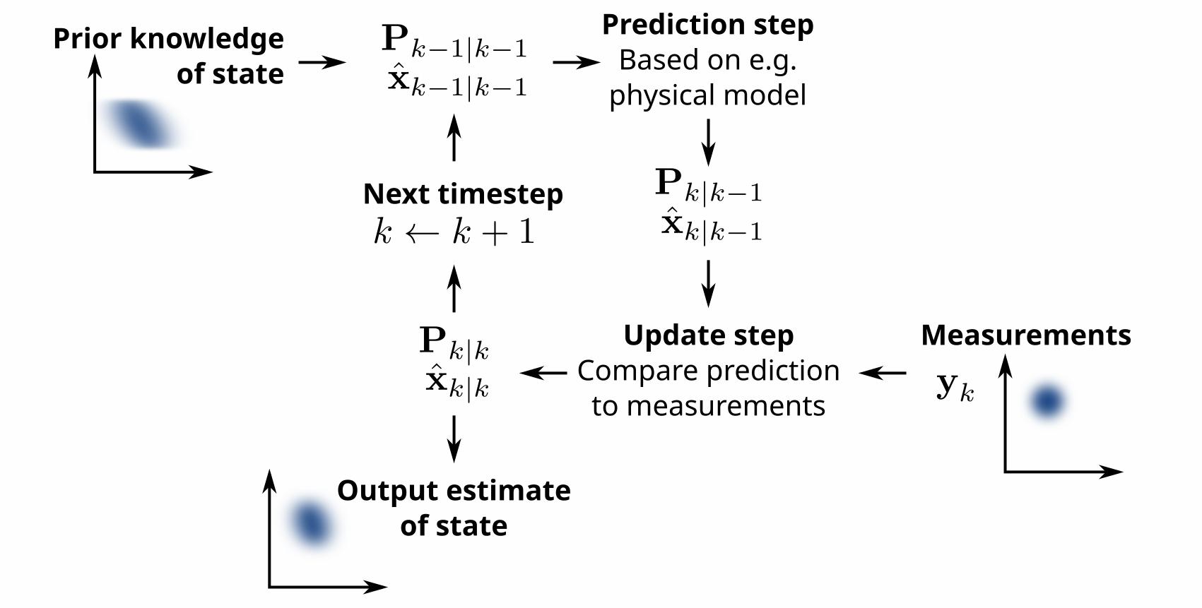
The underlying model:
$$\bf{z_k} = \bf{H}_k\bf{x}_k + \bf{v}_k$$
- $\bf{F}_k~\bf{x}_{k-1}$ is the AR part of the model
- $\bf{B}_k~\bf{u}_k$ is the command and how it impacts the system (control theory)
- $\bf{w}_k$ is the noise component
- Kalman filters can feel more suitable for systems on which we (as modelers) have some knowledge and hypothesis (control theory, Newtonian physics system)
Particle Filering
TODO
Practical Example
TODO